Chapter 2 Background on the SAPA Project
2.1 Packages
library(qgraph)
library(bootnet)
library(ggplot2)
library(psych)
library(RColorBrewer)
library(knitr)
library(kableExtra)
library(parallel)
library(broom)
library(igraph)
library(gridExtra)
library(data.table)
library(plyr)
library(tidyverse)
2.2 Methods
All of the data being pulled in have previously been cleaned. There are two big files — one from 2006 to 2010 and a second from 2010 to now.
2.2.1 2006 to 2010
The older data set is based on the predecessor platform to SAPA (a 50-item survey, created by William Revelle and hosted at www.personalityproject.org). There are a couple of issues with this sample. First, there was much less demographic information collected at that time (age, gender, ethnicity, education, and a few others). Second, it only sampled 50 items from the IPIP100 (each participant got 2 of 4 25-item blocks) and a preliminary set of ICAR items, most of which have since been deprecated. Third, there were two technical problems that caused a complete lack of data collection for one of the IPIP items (q_55) and a partial lack of data collection for two others (q_316 and q_995). Still, these data remain quite useful in that they include responses on 99 of the 100 IPIP items from about 114k participants.
The following code chunk pulls in the first sample and describes it. Note that only 99 variables are listed because item q_55 is empty.
data_path <- "https://github.com/emoriebeck/age_nets/blob/master"
load(url(sprintf("%s/data/SAPAdata4apr2006to18aug2010.rdata?raw=true", data_path)))

dim(taFinal)  # Participants who did not answer any IPIP100 items removed.
## [1] 114016 141# Identify Ps who didnt answer any IPIP100 items
empty <- rowSums(subset(taFinal, select = c(q_76:q_1989)), na.rm = TRUE)
taFinal <- taFinal[empty > 0, ]
dim(taFinal) # Participants who did not answer any IPIP100 items removed.## [1] 113961 141describe(subset(taFinal, select = c(q_76:q_1989)), fast = TRUE)## vars n mean sd min max range se
## q_76 1 56860 4.20 1.27 1 6 5 0.01
## q_108 2 56739 3.29 1.45 1 6 5 0.01
## q_124 3 56014 4.48 1.22 1 6 5 0.01
## q_128 4 55964 4.81 1.13 1 6 5 0.00
## q_132 5 57010 4.77 1.09 1 6 5 0.00
## q_140 6 56719 3.41 1.65 1 6 5 0.01
## q_146 7 56131 2.30 1.34 1 6 5 0.01
## q_150 8 56781 4.89 1.16 1 6 5 0.00
## q_177 9 56719 3.41 1.49 1 6 5 0.01
## q_194 10 56665 2.47 1.33 1 6 5 0.01
## q_195 11 56813 2.52 1.36 1 6 5 0.01
## q_200 12 56783 2.29 1.29 1 6 5 0.01
## q_217 13 57159 4.73 1.22 1 6 5 0.01
## q_240 14 56685 4.86 1.04 1 6 5 0.00
## q_241 15 56739 3.95 1.57 1 6 5 0.01
## q_248 16 56715 4.05 1.34 1 6 5 0.01
## q_254 17 57135 4.33 1.37 1 6 5 0.01
## q_262 18 56926 3.28 1.51 1 6 5 0.01
## q_316 19 5723 2.71 1.54 1 6 5 0.02
## q_403 20 57115 3.83 1.54 1 6 5 0.01
## q_422 21 57012 4.66 1.18 1 6 5 0.00
## q_492 22 55996 4.42 1.19 1 6 5 0.01
## q_493 23 57076 4.97 1.05 1 6 5 0.00
## q_497 24 56707 3.52 1.53 1 6 5 0.01
## q_530 25 56043 4.27 1.30 1 6 5 0.01
## q_609 26 56727 2.14 1.33 1 6 5 0.01
## q_619 27 56025 4.30 1.27 1 6 5 0.01
## q_626 28 56009 2.65 1.38 1 6 5 0.01
## q_690 29 56718 3.84 1.48 1 6 5 0.01
## q_698 30 56739 3.74 1.62 1 6 5 0.01
## q_712 31 56031 2.94 1.60 1 6 5 0.01
## q_815 32 57031 4.33 1.32 1 6 5 0.01
## q_819 33 56746 4.35 1.35 1 6 5 0.01
## q_838 34 56689 2.18 1.35 1 6 5 0.01
## q_844 35 56669 4.68 1.22 1 6 5 0.01
## q_890 36 57094 2.89 1.49 1 6 5 0.01
## q_901 37 56065 3.24 1.56 1 6 5 0.01
## q_904 38 57159 3.23 1.55 1 6 5 0.01
## q_931 39 56644 3.92 1.48 1 6 5 0.01
## q_952 40 56020 2.92 1.52 1 6 5 0.01
## q_960 41 57004 3.71 1.42 1 6 5 0.01
## q_962 42 56794 3.34 1.54 1 6 5 0.01
## q_974 43 56025 3.50 1.50 1 6 5 0.01
## q_979 44 57034 3.64 1.59 1 6 5 0.01
## q_986 45 56862 3.73 1.56 1 6 5 0.01
## q_995 46 5795 3.27 1.53 1 6 5 0.02
## q_1020 47 56943 3.51 1.39 1 6 5 0.01
## q_1041 48 57064 4.23 1.28 1 6 5 0.01
## q_1050 49 56791 4.36 1.30 1 6 5 0.01
## q_1053 50 56750 4.71 1.27 1 6 5 0.01
## q_1058 51 56700 4.84 1.20 1 6 5 0.01
## q_1083 52 56637 1.97 1.15 1 6 5 0.00
## q_1088 53 56773 2.49 1.32 1 6 5 0.01
## q_1090 54 56684 4.74 1.00 1 6 5 0.00
## q_1099 55 56135 3.23 1.58 1 6 5 0.01
## q_1114 56 56753 2.61 1.46 1 6 5 0.01
## q_1162 57 55998 4.83 1.13 1 6 5 0.00
## q_1163 58 56879 2.45 1.44 1 6 5 0.01
## q_1180 59 56738 3.35 1.45 1 6 5 0.01
## q_1205 60 56018 3.99 1.32 1 6 5 0.01
## q_1206 61 55916 4.59 1.28 1 6 5 0.01
## q_1254 62 57066 3.76 1.76 1 6 5 0.01
## q_1255 63 56782 3.37 1.67 1 6 5 0.01
## q_1290 64 56684 4.43 1.33 1 6 5 0.01
## q_1333 65 57010 4.08 1.50 1 6 5 0.01
## q_1364 66 56038 4.67 1.45 1 6 5 0.01
## q_1374 67 57062 4.16 1.38 1 6 5 0.01
## q_1385 68 57084 4.95 1.09 1 6 5 0.00
## q_1388 69 57056 4.01 1.60 1 6 5 0.01
## q_1392 70 57003 4.58 1.20 1 6 5 0.01
## q_1397 71 56715 2.73 1.41 1 6 5 0.01
## q_1410 72 56209 4.39 1.44 1 6 5 0.01
## q_1419 73 56077 4.61 1.18 1 6 5 0.00
## q_1422 74 57075 4.21 1.31 1 6 5 0.01
## q_1452 75 56685 2.28 1.31 1 6 5 0.01
## q_1479 76 55972 3.15 1.53 1 6 5 0.01
## q_1480 77 56834 3.06 1.50 1 6 5 0.01
## q_1483 78 56770 3.27 1.67 1 6 5 0.01
## q_1505 79 56005 3.00 1.59 1 6 5 0.01
## q_1507 80 56784 4.74 1.16 1 6 5 0.00
## q_1585 81 56738 3.24 1.45 1 6 5 0.01
## q_1677 82 56695 3.36 1.49 1 6 5 0.01
## q_1683 83 56629 3.61 1.52 1 6 5 0.01
## q_1696 84 56533 2.61 1.34 1 6 5 0.01
## q_1705 85 57010 4.99 0.98 1 6 5 0.00
## q_1738 86 56067 4.90 1.14 1 6 5 0.00
## q_1742 87 56672 4.27 1.39 1 6 5 0.01
## q_1763 88 56749 4.85 1.15 1 6 5 0.00
## q_1768 89 56005 4.33 1.31 1 6 5 0.01
## q_1775 90 57002 3.32 1.48 1 6 5 0.01
## q_1792 91 56656 4.65 1.12 1 6 5 0.00
## q_1803 92 56724 3.65 1.68 1 6 5 0.01
## q_1832 93 57047 4.30 1.25 1 6 5 0.01
## q_1861 94 56664 2.66 1.42 1 6 5 0.01
## q_1893 95 56675 3.64 1.49 1 6 5 0.01
## q_1913 96 57047 3.09 1.40 1 6 5 0.01
## q_1949 97 56037 3.44 1.56 1 6 5 0.01
## q_1964 98 55945 2.51 1.29 1 6 5 0.01
## q_1989 99 56748 4.36 1.40 1 6 5 0.01# table by gender
table(taFinal$gender)##
## Male Female
## 37864 76097# describe the age distribution
describe(taFinal$age, fast = TRUE)## vars n mean sd min max range se
## X1 1 113961 27.3 11.17 14 90 76 0.03# how many countries are represented?
length(table(taFinal$country))## [1] 204# show the top 25 countries
sort(table(taFinal$country), decreasing = TRUE)[1:25]##
## USA CAN GBR AUS IND MYS PHL CHN DEU SGP SWE MEX
## 83110 5661 4025 3647 1795 844 756 645 628 617 574 556
## POL NLD IRL NZL ZAF KOR HKG BRA NOR FRA ROU PAK
## 473 453 417 398 398 352 343 317 314 304 301 235
## ITA
## 215# show the US states, in order
sort(table(taFinal$state), decreasing = TRUE)[1:51]##
## California Illinois New York
## 9709 5520 4942
## Pennsylvania Texas Ohio
## 4758 4662 3600
## Florida Virginia Michigan
## 2936 2787 2549
## New Jersey Georgia Wisconsin
## 2495 2414 2377
## Minnesota Louisiana Massachusetts
## 2104 2030 1935
## Maryland Washington Indiana
## 1772 1742 1707
## Missouri North Carolina Oregon
## 1611 1454 1203
## New Mexico Tennessee Colorado
## 1199 1133 1097
## South Carolina Connecticut Iowa
## 1010 986 982
## Arizona Kentucky Kansas
## 866 820 808
## Oklahoma Alabama Mississippi
## 771 643 604
## Delaware Nebraska Arkansas
## 592 580 577
## Alaska Utah Rhode Island
## 555 487 422
## New Hampshire West Virginia Maine
## 389 384 356
## Idaho Hawaii Nevada
## 340 292 274
## Montana North Dakota District of Columbia
## 243 190 174
## South Dakota Vermont Wyoming
## 172 161 126# table by ethnicity
table(taFinal$ethnic)## < table of extent 0 ># table by education
table(taFinal$education)##
## Less than 12 years High school graduate
## 15052 9037
## Some college did not graduate Currently attending college
## 10736 42080
## College graduate Graduate or professional degree
## 18296 187602.2.2 2010 to 2017}
From August 18, 2010 to February 7, 2017, the data were collected from the SAPA-Project.org. While many more variables (including many more demographic variables) were collected in this sample, the data are pared down to match the older set. It should also be noted that large subsets of these data have previously been placed in the public domain (see https://dataverse.harvard.edu/dataverse/SAPA-Project).
Here, we pull in the second sample, subset it, and describe the result.
load(url(sprintf("%s/data/SAPAdata18aug2010thru7feb2017.rdata?raw=true", data_path)))

dim(SAPAdata18aug2010thru7feb2017)  # Participants who did not answer any IPIP100 items removed.
## [1] 255348 953# Identify Ps who didnt answer any IPIP100 items
empty <- rowSums(subset(SAPAdata18aug2010thru7feb2017, select = c(q_55:q_1989)),
na.rm = TRUE)
SAPAdata18aug2010thru7feb2017 <- SAPAdata18aug2010thru7feb2017[empty > 0, ]
dim(SAPAdata18aug2010thru7feb2017) # Participants who did not answer any IPIP100 items removed.## [1] 255190 953SAPAdata18aug2010thru7feb2017 <- SAPAdata18aug2010thru7feb2017 %>% select(one_of(c("q_55",
colnames(taFinal)))) %>% select(RID:education, q_55, everything())
describe(subset(SAPAdata18aug2010thru7feb2017, select = c(q_55:q_1989)), fast = TRUE)## vars n mean sd min max range se
## q_55 1 59248 4.05 1.49 1 6 5 0.01
## q_76 2 59282 4.18 1.26 1 6 5 0.01
## q_108 3 57880 3.21 1.45 1 6 5 0.01
## q_124 4 70237 4.45 1.18 1 6 5 0.00
## q_128 5 69812 4.77 1.14 1 6 5 0.00
## q_132 6 69751 4.64 1.15 1 6 5 0.00
## q_140 7 59834 3.41 1.63 1 6 5 0.01
## q_146 8 68259 2.38 1.36 1 6 5 0.01
## q_150 9 68308 4.81 1.19 1 6 5 0.00
## q_177 10 58340 3.44 1.49 1 6 5 0.01
## q_194 11 59219 2.43 1.31 1 6 5 0.01
## q_195 12 68069 2.61 1.38 1 6 5 0.01
## q_200 13 68525 2.41 1.33 1 6 5 0.01
## q_217 14 59074 4.70 1.21 1 6 5 0.00
## q_240 15 69644 4.82 1.05 1 6 5 0.00
## q_241 16 59522 4.01 1.58 1 6 5 0.01
## q_248 17 58209 4.00 1.37 1 6 5 0.01
## q_254 18 60182 4.21 1.41 1 6 5 0.01
## q_262 19 59494 3.18 1.54 1 6 5 0.01
## q_316 20 69979 2.70 1.54 1 6 5 0.01
## q_403 21 59382 3.98 1.53 1 6 5 0.01
## q_422 22 69499 4.61 1.21 1 6 5 0.00
## q_492 23 69740 4.41 1.20 1 6 5 0.00
## q_493 24 69509 4.91 1.06 1 6 5 0.00
## q_497 25 58027 3.44 1.52 1 6 5 0.01
## q_530 26 70916 4.31 1.27 1 6 5 0.00
## q_609 27 59701 2.19 1.36 1 6 5 0.01
## q_619 28 70528 4.31 1.25 1 6 5 0.00
## q_626 29 59498 2.59 1.35 1 6 5 0.01
## q_690 30 59601 3.96 1.48 1 6 5 0.01
## q_698 31 70353 3.54 1.61 1 6 5 0.01
## q_712 32 59897 3.05 1.61 1 6 5 0.01
## q_815 33 59519 4.20 1.36 1 6 5 0.01
## q_819 34 59304 4.27 1.39 1 6 5 0.01
## q_838 35 68245 2.35 1.46 1 6 5 0.01
## q_844 36 68357 4.68 1.23 1 6 5 0.00
## q_890 37 58185 2.89 1.47 1 6 5 0.01
## q_901 38 59862 3.27 1.58 1 6 5 0.01
## q_904 39 59520 3.21 1.54 1 6 5 0.01
## q_931 40 70518 4.02 1.45 1 6 5 0.01
## q_952 41 58427 2.92 1.52 1 6 5 0.01
## q_960 42 58032 3.70 1.44 1 6 5 0.01
## q_962 43 59196 3.37 1.54 1 6 5 0.01
## q_974 44 58193 3.49 1.49 1 6 5 0.01
## q_979 45 58197 3.62 1.59 1 6 5 0.01
## q_986 46 58344 3.79 1.57 1 6 5 0.01
## q_995 47 58004 3.25 1.52 1 6 5 0.01
## q_1020 48 58039 3.42 1.39 1 6 5 0.01
## q_1041 49 68142 4.30 1.26 1 6 5 0.00
## q_1050 50 69752 4.34 1.29 1 6 5 0.00
## q_1053 51 68453 4.70 1.26 1 6 5 0.00
## q_1058 52 59526 4.81 1.21 1 6 5 0.00
## q_1083 53 59048 2.00 1.17 1 6 5 0.00
## q_1088 54 69366 2.48 1.30 1 6 5 0.00
## q_1090 55 69251 4.67 1.03 1 6 5 0.00
## q_1099 56 58276 3.19 1.56 1 6 5 0.01
## q_1114 57 59641 2.72 1.47 1 6 5 0.01
## q_1162 58 68437 4.79 1.16 1 6 5 0.00
## q_1163 59 58733 2.40 1.41 1 6 5 0.01
## q_1180 60 59365 3.47 1.47 1 6 5 0.01
## q_1205 61 69960 3.92 1.34 1 6 5 0.01
## q_1206 62 68167 4.57 1.28 1 6 5 0.00
## q_1254 63 59382 3.71 1.73 1 6 5 0.01
## q_1255 64 59350 3.33 1.64 1 6 5 0.01
## q_1290 65 70597 4.49 1.27 1 6 5 0.00
## q_1333 66 69656 4.15 1.46 1 6 5 0.01
## q_1364 67 68534 4.63 1.47 1 6 5 0.01
## q_1374 68 70631 4.25 1.33 1 6 5 0.01
## q_1385 69 68461 5.01 1.09 1 6 5 0.00
## q_1388 70 69687 3.98 1.58 1 6 5 0.01
## q_1392 71 69585 4.58 1.20 1 6 5 0.00
## q_1397 72 59299 2.82 1.42 1 6 5 0.01
## q_1410 73 59784 4.30 1.47 1 6 5 0.01
## q_1419 74 68562 4.61 1.16 1 6 5 0.00
## q_1422 75 59488 4.27 1.29 1 6 5 0.01
## q_1452 76 59530 2.31 1.32 1 6 5 0.01
## q_1479 77 58257 3.17 1.53 1 6 5 0.01
## q_1480 78 59220 3.11 1.51 1 6 5 0.01
## q_1483 79 59564 3.29 1.64 1 6 5 0.01
## q_1505 80 58229 3.05 1.60 1 6 5 0.01
## q_1507 81 70717 4.80 1.13 1 6 5 0.00
## q_1585 82 58116 3.23 1.44 1 6 5 0.01
## q_1677 83 58010 3.27 1.49 1 6 5 0.01
## q_1683 84 58091 3.62 1.50 1 6 5 0.01
## q_1696 85 58914 2.60 1.34 1 6 5 0.01
## q_1705 86 68148 4.99 1.01 1 6 5 0.00
## q_1738 87 59777 4.93 1.13 1 6 5 0.00
## q_1742 88 59128 4.15 1.43 1 6 5 0.01
## q_1763 89 68336 4.83 1.18 1 6 5 0.00
## q_1768 90 70279 4.33 1.31 1 6 5 0.00
## q_1775 91 58307 3.19 1.48 1 6 5 0.01
## q_1792 92 68363 4.68 1.14 1 6 5 0.00
## q_1803 93 59615 3.55 1.70 1 6 5 0.01
## q_1832 94 68502 4.43 1.25 1 6 5 0.00
## q_1861 95 59797 2.72 1.43 1 6 5 0.01
## q_1893 96 59820 3.73 1.46 1 6 5 0.01
## q_1913 97 70046 3.08 1.41 1 6 5 0.01
## q_1949 98 59504 3.39 1.57 1 6 5 0.01
## q_1964 99 59480 2.46 1.25 1 6 5 0.01
## q_1989 100 58160 4.43 1.40 1 6 5 0.01# table by gender
table(SAPAdata18aug2010thru7feb2017$gender)##
## male female
## 95169 160020# describe the age distribution
describe(SAPAdata18aug2010thru7feb2017$age, fast = TRUE)## vars n mean sd min max range se
## X1 1 255190 25.94 10.73 14 90 76 0.02# how many countries are represented?
length(table(SAPAdata18aug2010thru7feb2017$country))## [1] 220# show the top 25 countries
sort(table(SAPAdata18aug2010thru7feb2017$country), decreasing = TRUE)[1:25]##
## USA CAN GBR AUS IND SWE DEU PHL MYS CHN
## 168816 10581 7214 4790 2782 2425 2346 2239 2151 1441
## NLD SGP NOR NZL MEX FRA BRA ZAF FIN IRL
## 1301 1269 1170 1033 984 844 830 793 772 673
## IDN POL ROU HKG ITA
## 646 641 623 576 568# show the US states, in order
state <- subset(SAPAdata18aug2010thru7feb2017, country == "USA")
sort(table(state$state), decreasing = TRUE)[1:51]##
## California Illinois Texas
## 18062 11611 10367
## New York Florida Pennsylvania
## 8882 8054 7919
## Michigan Ohio Virginia
## 7660 6213 5763
## Georgia Washington Minnesota
## 5308 4753 4090
## North Carolina Wisconsin New Jersey
## 3607 3394 3290
## Massachusetts Indiana Maryland
## 3147 2938 2689
## Missouri Arizona Louisiana
## 2567 2495 2487
## South Carolina New Mexico Oregon
## 2479 2223 2213
## Tennessee Delaware Alabama
## 2135 1929 1865
## Colorado Kentucky Oklahoma
## 1816 1757 1643
## Iowa Connecticut Nebraska
## 1441 1355 1348
## Utah Kansas Mississippi
## 1309 1165 978
## Arkansas Rhode Island Nevada
## 925 825 763
## Idaho New Hampshire Alaska
## 683 611 578
## Maine Montana West Virginia
## 576 553 512
## Hawaii South Dakota Vermont
## 487 401 312
## District of Columbia North Dakota Wyoming
## 309 268 216# table by ethnicity
table(SAPAdata18aug2010thru7feb2017$ethnic)## < table of extent 0 ># table by education
table(SAPAdata18aug2010thru7feb2017$education)##
## less12yrs HSgrad CurrentInUniv SomeCollege
## 33011 17517 104783 13006
## CollegeDegree InGradOrProSchool GradOrProDegree
## 32020 11431 191992.2.3 Merge the datasets and Describe}
Now we will combine both of the samples and describe them with proper tables and figures before converting the demographics into numeric variables.
fullSample <- taFinal %>% select(-contains("iq_")) %>% full_join(SAPAdata18aug2010thru7feb2017) %>%
    select(RID:education, q_55, everything())

rm(SAPAdata18aug2010thru7feb2017, taFinal)
gc()
## used (Mb) gc trigger (Mb) limit (Mb) max used (Mb)
## Ncells 4507029 240.8 10045189 536.5 NA 10045189 536.5
## Vcells 107160950 817.6 392190552 2992.2 51200 490231665 3740.2# n is total Ps in the full sample
n <- dim(fullSample)[1]
ntext <- prettyNum(n, big.mark = ",", scientific = F)
ntext## [1] "369,151"# percent female
femalePerc <- 100 * round((table(fullSample$gender)/sum(table(fullSample$gender)))["female"],
3)
femalePerc## female
## 43.3# describe the age distribution
(fullSampleAge <- psych::describe(fullSample[, "age"]))## vars n mean sd median trimmed mad min max range skew kurtosis
## X1 1 369151 26.36 10.89 22 24.53 7.41 14 90 76 1.48 1.86
## se
## X1 0.02(MeanAge <- fullSampleAge$mean)## [1] 26.36206(SDAge <- fullSampleAge$sd)## [1] 10.88535(MedianAge <- fullSampleAge$median)## [1] 22(MinAge <- fullSampleAge$min)## [1] 14(MaxAge <- fullSampleAge$max)## [1] 90# percent U.S.
(USperc <- 100 * round((table(fullSample$country)/sum(table(fullSample$country)))["USA"],
3))## USA
## 72.5# total U.S.
(UScounttext <- prettyNum((table(fullSample$country))["USA"], big.mark = ",",
scientific = F))## USA
## "251,926"# number of countries with P>0
countryTable <- sort(table(fullSample$country), decreasing = TRUE)
countryCount <- length(countryTable)
# number of countries with P>199
countryCount200 <- subset(countryTable, countryTable > 199)
length(countryCount200)## [1] 67# show the top 25 countries
sort(table(fullSample$country), decreasing = TRUE)[1:25]##
## USA CAN GBR AUS IND SWE MYS PHL DEU CHN
## 251926 16242 11239 8437 4577 2999 2995 2995 2974 2086
## SGP NLD MEX NOR NZL ZAF FRA BRA POL IRL
## 1886 1754 1540 1484 1431 1191 1148 1147 1114 1090
## FIN ROU HKG IDN ITA
## 963 924 919 847 783(countrytext <- prettyNum(sum(table(fullSample$country)), big.mark = ",", scientific = F))## [1] "347,672"# show the US states, in order
state <- subset(fullSample, country == "USA")
sort(table(state$state), decreasing = TRUE)[1:51]##
## California Illinois Texas
## 27771 17131 15029
## New York Pennsylvania Florida
## 13824 12677 10990
## Michigan Ohio Virginia
## 10209 9813 8550
## Georgia Washington Minnesota
## 7722 6495 6194
## New Jersey Wisconsin Massachusetts
## 5785 5771 5082
## North Carolina Indiana Louisiana
## 5061 4645 4517
## Maryland Missouri South Carolina
## 4461 4178 3489
## New Mexico Oregon Arizona
## 3422 3416 3361
## Tennessee Colorado Kentucky
## 3268 2913 2577
## Delaware Alabama Iowa
## 2521 2508 2423
## Oklahoma Connecticut Kansas
## 2414 2341 1973
## Nebraska Utah Mississippi
## 1928 1796 1582
## Arkansas Rhode Island Alaska
## 1502 1247 1133
## Nevada Idaho New Hampshire
## 1037 1023 1000
## Maine West Virginia Montana
## 932 896 796
## Hawaii South Dakota District of Columbia
## 779 573 483
## Vermont North Dakota Wyoming
## 473 458 342education <- data.frame(table(fullSample$education))
colnames(education) <- c("Educational Level", "Participants")
(college <- prettyNum(round(education[4, 2]/sum(education[, 2]) * 100, 0), big.mark = ",",
scientific = F))## [1] "12"ethnic <- data.frame(table(fullSample$race))
colnames(ethnic) <- c("Ethnicity/Race", "Participants")fullSample <- IPIP100items04apr2006thru7feb2017
fullSample %>%
filter(!is.na(country)) %>%
group_by(country) %>%
summarize(n = n()) %>%
arrange(desc(n)) %>%
filter(row_number() %in% 1:25) %>%
kable(., "html", booktabs = T, escape = F,
caption = "Sample Sizes in Top 25 Countries",
col.names = c("Country", "Frequency")) %>%
kable_styling(full_width = F)| Country | Frequency |
|---|---|
| USA | 251913 |
| CAN | 16242 |
| GBR | 11237 |
| AUS | 8437 |
| IND | 4576 |
| SWE | 2999 |
| MYS | 2995 |
| PHL | 2994 |
| DEU | 2974 |
| CHN | 2086 |
| SGP | 1885 |
| NLD | 1754 |
| MEX | 1540 |
| NOR | 1484 |
| NZL | 1430 |
| ZAF | 1191 |
| FRA | 1148 |
| BRA | 1147 |
| POL | 1114 |
| IRL | 1090 |
| FIN | 963 |
| ROU | 924 |
| HKG | 919 |
| IDN | 847 |
| ITA | 782 |
ethnic %>%
  arrange(desc(Participants)) %>%
  kable(., "html", booktabs = T, escape = F,
        caption = "Race/Ethnicity Among U.S. Participants in the full sample") %>%
kable_styling(full_width = F)| Ethnicity/Race | Participants |
|---|---|
| White/Caucasian | 63763 |
| African American | 6354 |
| Other | 3201 |
| Mexican | 2249 |
| Latino | 2184 |
| Chinese | 1189 |
| Native American | 741 |
| Philipino | 649 |
| Other Asian | 597 |
| Puerto Rican | 555 |
| Korean | 528 |
| Indian/Pakistani | 498 |
| Pacific Islander | 329 |
| Japanese | 266 |
levs <- tibble(old = c("less12yrs", "Less than 12 years", "HSgrad", "High school graduate", "SomeCollege",
                 "Some college did not graduate", "CurrentInUniv", "Currently attending college",
                 "CollegeDegree", "College graduate", "InGradOrProSchool", "Graduate or professional degree",
                 "GradOrProDegree"),
               new = c(rep("Less than 12 years", 2), rep("High school graduate", 2),
                       rep("Some college/university, but did not graduate", 2),
                       rep("Currently in college/university", 2), rep("College/university degree", 2),
                       "Currently in graduate or professional school",
                       rep("Graduate or professional school degree", 2)))
education %>%
  mutate(`Educational Level` = mapvalues(`Educational Level`, levs$old, levs$new)) %>%
  group_by(`Educational Level`) %>%
  summarize(Participants = sum(Participants)) %>%
  ungroup() %>%
  mutate(`Educational Level` = factor(`Educational Level`, levels = unique(levs$new))) %>%
  arrange(`Educational Level`) %>%
  kable(., "html", booktabs = T, escape = F,
        caption = "Educational Attainment Level in the full sample") %>%
kable_styling(full_width = F)| Educational Level | Participants |
|---|---|
| Less than 12 years | 48063 |
| High school graduate | 26554 |
| Some college/university, but did not graduate | 23742 |
| Currently in college/university | 146863 |
| College/university degree | 50316 |
| Currently in graduate or professional school | 11431 |
| Graduate or professional school degree | 37959 |
It’s also useful to describe the extent of the missingness in the data (for the IPIP100 variables) and the number of pairwise administrations across the items. While we’re at it, we’ll also bootstrap estimates of the standard errors of the item-level correlations.
items <- colnames(subset(fullSample, select = c(q_55:q_1989)))

not_na_count <- apply(fullSample[,items], 1, function(x) sum(!is.na(x)))

partAdminsMean <- round(mean(not_na_count), 0)
partAdminsMean <- prettyNum(partAdminsMean, big.mark=",", scientific=F)

partAdminsMedian <- round(median(not_na_count), 0)
partAdminsMedian <- prettyNum(partAdminsMedian, big.mark=",", scientific=F)

partAdminsSD <- round(sd(not_na_count), 0)
partAdminsSD <- prettyNum(partAdminsSD, big.mark=",", scientific=F)

described <- describe(fullSample[,items])

AdminsMean <- round(mean(described$n), 0)
AdminsMean <- prettyNum(AdminsMean, big.mark=",", scientific=F)

AdminsMedian <- round(median(described$n), 0)
AdminsMedian <- prettyNum(AdminsMedian, big.mark=",", scientific=F)

AdminsSD <- round(sd(described$n), 0)
AdminsSD <- prettyNum(AdminsSD, big.mark=",", scientific=F)

# The mean, median and sd of administrations of items
AdminsMean
AdminsMedian
AdminsSD
rm(described)

pwiseAdmins1 <- pairwiseDescribe(fullSample[,items])
pwiseAdmins <- prettyNum(pwiseAdmins1, big.mark=",", scientific=F)

pwiseAdminsMean <- round(pwiseAdmins1$mean, 0)
pwiseAdminsMean <- prettyNum(pwiseAdminsMean, big.mark=",", scientific=F)

pwiseAdminsMedian <- round(pwiseAdmins1$median, 0)
pwiseAdminsMedian <- prettyNum(pwiseAdminsMedian, big.mark=",", scientific=F)

pwiseAdminsSD <- round(pwiseAdmins1$sd, 0)
pwiseAdminsSD <- prettyNum(pwiseAdminsSD, big.mark=",", scientific=F)

pwiseAdminsMin <- round(pwiseAdmins1$min, 0)
pwiseAdminsMin <- prettyNum(pwiseAdminsMin, big.mark=",", scientific=F)

# The mean, median and sd of pairwise administrations of items
pwiseAdminsMean
pwiseAdminsMedian
pwiseAdminsSD

#rm(pwiseAdmins1)
# the CIs around the rs
IPIP100CorCI <- cor.ci(fullSample[,items], p=.05, n.iter = 100, overlap=FALSE, plot = FALSE, poly = FALSE)
save(IPIP100CorCI, file = "~/Downloads/cor_stab.RData")load(url(sprintf("%s/results/cor_stab.RData?raw=true", data_path)))
plot(density(IPIP100CorCI$sds), main="", ylab="Frequency", xlab="Standard error of item-level correlations", xlim= c(0,.02), ylim = c(0,1000))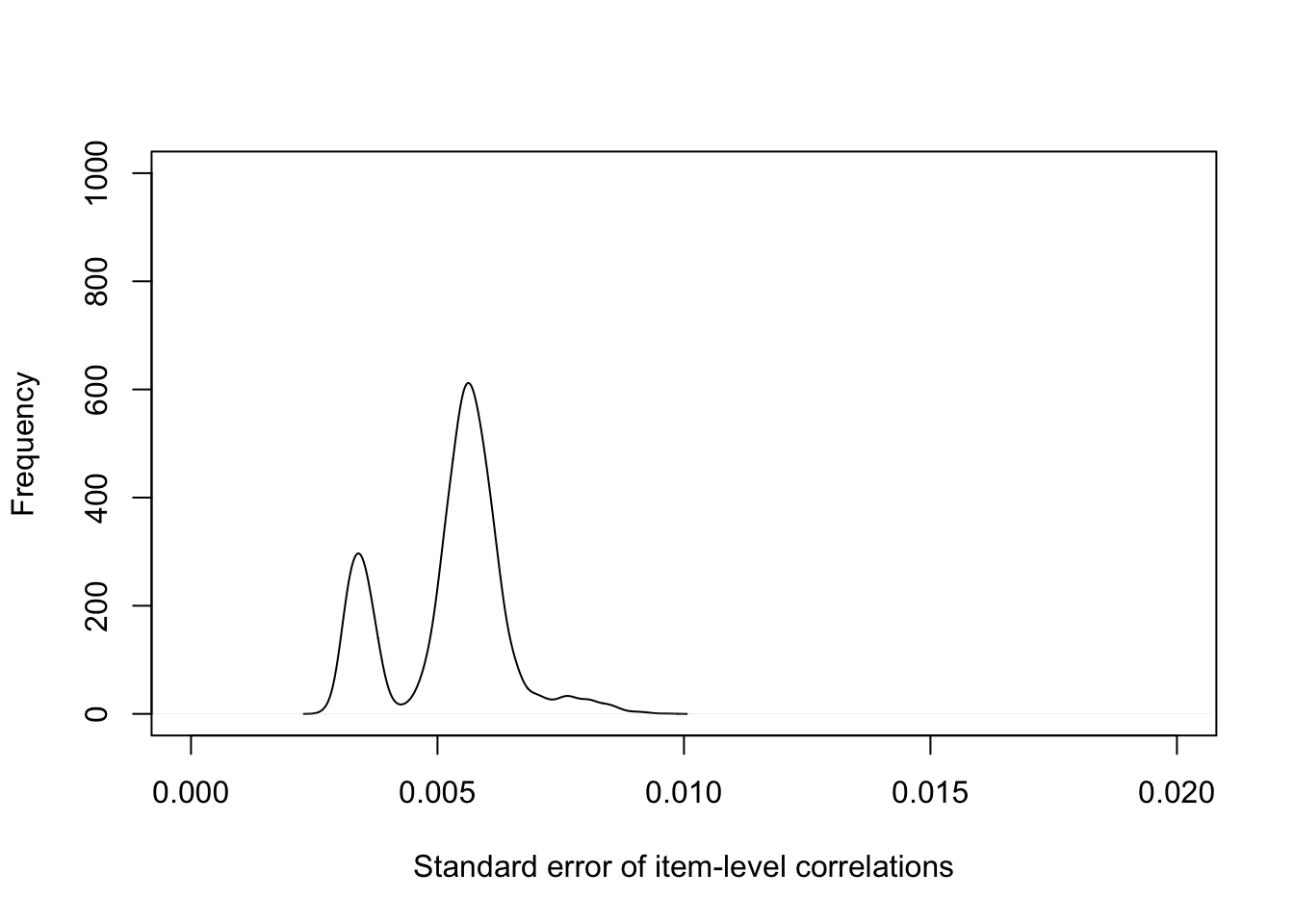
Figure 2.1: Supplementary Figure 2. Standard error of item-level correlations
Clean up some of the helper objects and save the data for further analysis later.
IPIP100items04apr2006thru7feb2017 <- fullSample

ItemInfo100 <- ItemInfo[items,1:2]

keys.list.trimmed <- keys.list[c("IPIP100agreeableness20","IPIP100conscientiousness20", "IPIP100extraversion20", "IPIP100intellect20", "IPIP100EmotionalStability20")]

ItemLists.trimmed <- ItemLists[c("IPIP100agreeableness20","IPIP100conscientiousness20", "IPIP100extraversion20", "IPIP100intellect20", "IPIP100EmotionalStability20")]

save(IPIP100items04apr2006thru7feb2017, ItemInfo100, ItemLists.trimmed, keys.list.trimmed, file=paste(filepathdata, "IPIP100items04apr2006thru7feb2017.rdata", sep=""))