Chapter 7 Community Structure

Next, we calculate the communities in each network using the Spin Glass algorithm. Although there is no widely accepted definition of communities (Baroncelli, 2012), communities are generally considered to be nodes that are more connected to each other than to other nodes. For demonstrative purposes, we separately collapse across the 20s and 60s and run the networks. Then we calculate their community structure and compare them. ## Multi-Trait ### Run Communities

communities_fun <-   function(g, cols){    
        g <- igraph::as.igraph(g)
        V(g)$label <- cols
        g2 <- g
        E(g2)$weight <- abs(E(g2)$weight)
        lvc <- igraph::cluster_louvain(g2)
        subgraphs <- list()
        for (i in 1:length(unique(lvc$membership))){
          subgraphs[[i]] <- igraph::induced_subgraph(g,
            vids = which(lvc$membership == i),
            impl = "copy_and_delete")}
        results <- list(graph = g, 
                        louvain = lvc,
                        subgraphs = subgraphs)
        return(results)
}

membership_fun <- function(comm, cols){
  comm <- comm$louvain$membership %>% setNames(cols)
}

MT_net_nested <- MT_net_nested %>%
  mutate(communities = map2(net, cols, communities_fun),
         membership = map2(communities, cols, possibly(membership_fun, NA_real_)))

MT_net_nested_gr <- MT_net_nested_gr %>%
  mutate(communities = map2(net, cols, communities_fun),
         membership = map2(communities, cols, membership_fun))

communitiesall <- (MT_net_nested %>% filter(inventory == "IPIP50"))$membership %>% ldply(.)
communities38below <- (MT_net_nested %>% filter(inventory == "IPIP50" & age <= 38))$membership %>% ldply(.)
communities39above <- (MT_net_nested %>% filter(inventory == "IPIP50" & age >= 39))$membership %>% ldply(.)

7.0.1 Plots

communities20s <- (MT_net_nested_gr %>% filter(inventory == "IPIP50" & age_group == 2))$communities[[1]]
communities60s <- (MT_net_nested_gr %>% filter(inventory == "IPIP50" & age_group == 6))$communities[[1]]

b_color_fun <- function(c){
  mapvalues(c$louvain$membership, from = seq(1, max(c$louvain$membership),1), 
            to = RColorBrewer::brewer.pal(max(c$louvain$membership),"Set3"))
}

MT_net_nested_gr <- MT_net_nested_gr %>%
  mutate(bordercolors = map(communities, b_color_fun), 
         net = map2(net, bordercolors, EDBqgraph_communities)) %>%
  arrange(age_group)

# pdf(filename = sprintf("%s/SAPA/photos/nets_20s_60s.bmp", data_path), width = 800, height = 400)
par(mfrow = c(1,2))
plot((MT_net_nested_gr %>% filter(inventory == "IPIP50" & age_group == 2))$net[[1]])
title("20s")
plot((MT_net_nested_gr %>% filter(inventory == "IPIP50" & age_group == 6))$net[[1]])
title("60s")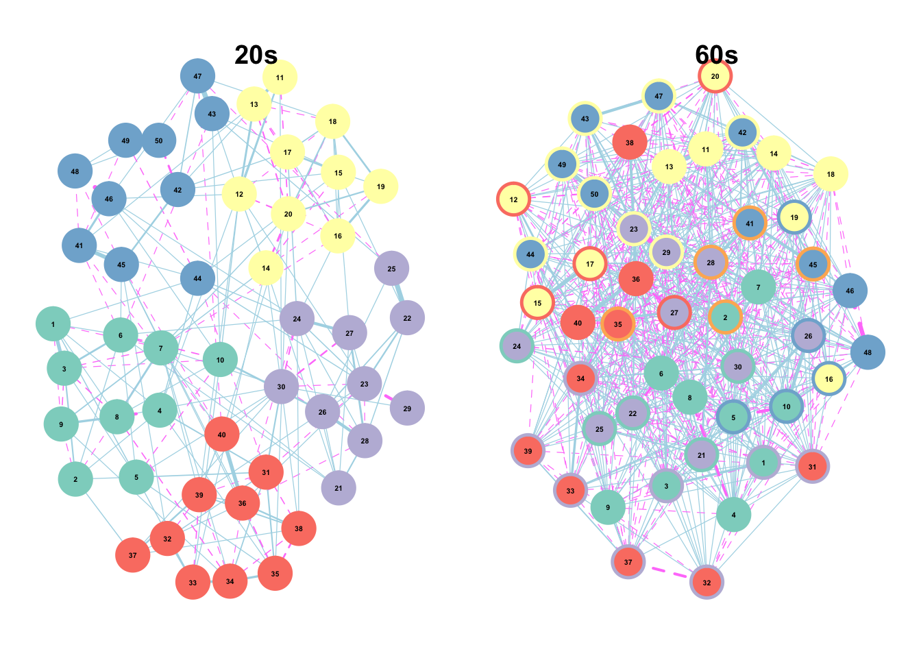

(#fig:comm plots)Figure 3. Item networks by age group. Nodes (circles) represent unique IPIP-50 items. Nodes colors are colored according to their putative Big Five scale membership, while node borders are colored according to their empirically derived community membership. Edges (lines between nodes) indicate partial correlations. Solid lines indicate positive relationships, while dashed lines indicate negative relationships.

# dev.off()

par(mfrow = c(2,4))
lapply(1:7, function(x){ plot((MT_net_nested_gr %>% filter(inventory == "IPIP50"))$net[[x]]); title(sprintf("%s0s", x))})

## [[1]]
## NULL
## 
## [[2]]
## NULL
## 
## [[3]]
## NULL
## 
## [[4]]
## NULL
## 
## [[5]]
## NULL
## 
## [[6]]
## NULL
## 
## [[7]]
## NULL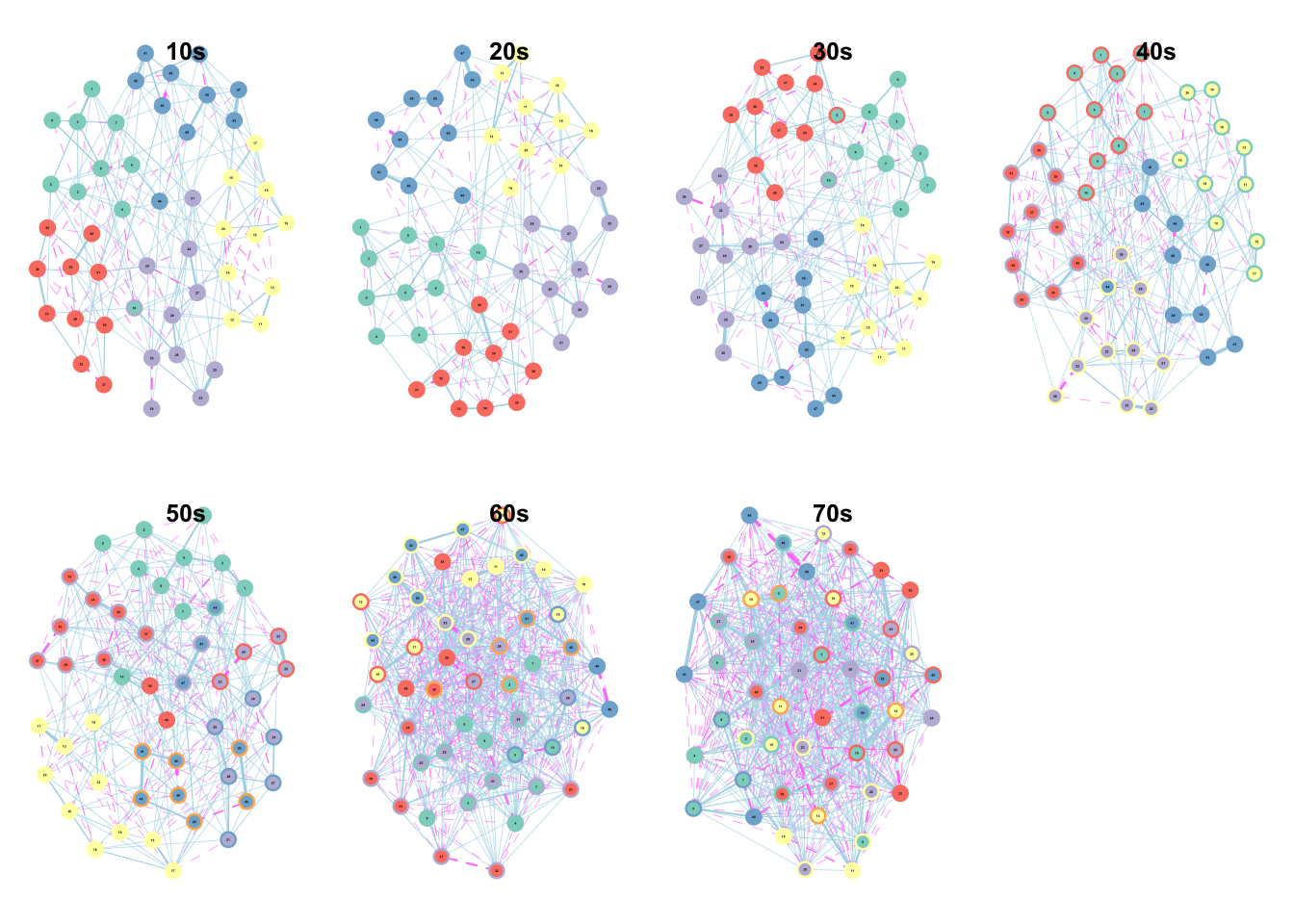

(#fig:age plots)Supplementary Figure 3. Network Structure by Decade

7.0.2 Matching Across Communities

The code below is a little incomprehensible, but in this instance there isn’t really a better alternative.

match_mat <- matrix(rep(NA, 50*50), nrow = 50)
for(i in 1:50){ # 
  for(j in 1:50){
    match <- 0L
    for(k in 1:50){
      match <- ifelse(communitiesall[k,i] == communitiesall[k,j], match + 1, match)
    }
    match_mat[i,j] <- match
  }
}

match_mat38below <- matrix(rep(NA, 50*50), nrow = 50)
match_mat39above <- matrix(rep(NA, 50*50), nrow = 50)
for(i in 1:50){
  for(j in 1:50){
    match38below <- 0L
    match39above <- 0L
    for(k in 1:25){
      match38below <- ifelse(communities38below[k,i] == communities38below[k,j], match38below + 1, match38below)
      match39above <- ifelse(communities39above[k,i] == communities39above[k,j], match39above + 1, match39above)
    }
    match_mat38below[i,j] <- match38below
    match_mat39above[i,j] <- match39above
  }
}

community_plot_fun <- function(df, age, lim){
  colnames(df) <- all_cols50; rownames(df) <- all_cols50
  df[upper.tri(df, diag = T)] <- NA
  tbl_df(df) %>%
    mutate(Edge1 = factor(all_cols50, levels = all_cols50)) %>%
    gather(key = Edge2, value = communities, 1:50) %>%
    mutate(Edge2 = factor(Edge2, levels = all_cols50)) %>%
    filter(!is.na(communities)) %>%
    ggplot(aes(x = Edge2, y = Edge1, fill = communities)) + 
      geom_raster() + 
      scale_fill_gradient(
        high = "orchid4", low = "white",
        limit = c(0,lim), name="Shared\nCommunity\nSums") +
        labs(x = NULL, y = NULL, 
             title = sprintf("%s", age)) + 
      theme_classic() + 
      theme(axis.text.x = element_text(face = "bold", angle = 90),
            axis.text.y = element_text(face = "bold"),
            plot.title = element_text(hjust = .5, face = "bold"))
}

communityall     <- community_plot_fun(match_mat, "All", 50) + theme(legend.position = c(.9, .5))
community38below <- community_plot_fun(match_mat38below, "38 & below", 25) + 
  theme(legend.position = "none",
        axis.text = element_text(size = rel(.3)))
community39above <- community_plot_fun(match_mat39above, "39 & above", 25) + 
  theme(legend.position = "none",
        axis.text = element_text(size = rel(.3)))

community_plot <-  grid.arrange(communityall, community38below, community39above, 
             layout_matrix = rbind(c(1,1,3),
                                   c(1,1,4)))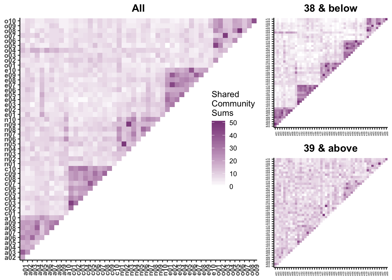

(#fig:comm plot)Figure 4. Frequency of shared community membership across items in (A) the full sample (B), participants 38 and below, (C) and participants 39 and above. Groups were split according to a median age split of all age groups for ease of comparing frequency, The diagonal of each plot indicates items within the same Big 5 scale, while off-diagonal elements are largely items of different scales. Darker colors indicate that the empirically derived community membership of two nodes was frequently shared across age groups, while lighter colors indicate that community membership was often not shared.

# ggsave(plot = community_plot, file = sprintf("%s/photos/shared_communities.png", data_path), 
#        width = 9, height = 6)