Chapter 6 Age Differences in Coherence and Differentiation

trait.edges.sum <- ST_net_nested %>%
  unnest(edges.df) %>%
  group_by(inventory, age, Trait) %>%
  summarize(mean = fisherz2r(mean(fisherz(abs(weight)), na.rm = T))) %>%
  ungroup() %>% group_by(age) %>%
  mutate(type = "Single Trait", comp = "ST-Coherence",
         gmean = fisherz2r(mean(fisherz(mean), na.rm = T)), 
         traits = Trait)

trait.edges.sum50 <- trait.edges.sum %>%
  filter(inventory == "IPIP50")
  
edges.sum <- MT_net_nested %>%
  unnest(edges.df) %>%
  separate(from, c("from_trait", "from_item"), 1) %>%
  separate(to, c("to_trait", "to_item"), 1) %>%
  unite(traits, from_trait, to_trait, remove = F) %>%
  mutate(comp = ifelse(from_trait == to_trait, "Coherence", "Differentiation")) %>%
  group_by(inventory, age, traits, comp, from_trait, to_trait) %>%
  summarize(n = n(), mean = fisherz2r(mean(fisherz(abs(weight)), na.rm = T))) %>%
  ungroup() %>% group_by(inventory, age, from_trait, comp) %>%
  mutate(traitMean1 = fisherz2r(mean(fisherz(mean), na.rm = T))) %>%
  ungroup() %>% group_by(inventory, age, to_trait, comp) %>%
  mutate(traitMean2 = fisherz2r(mean(fisherz(mean), na.rm = T))) %>%
  ungroup() %>% 
  mutate(traitMean = fisherz2r(rowMeans(cbind(fisherz(traitMean1), fisherz(traitMean2)), na.rm = T))) %>%
  ungroup() %>% group_by(inventory, age, comp) %>%
  mutate(type = "Multi Trait", 
         gmean = fisherz2r(mean(fisherz(mean), na.rm = T))) %>%
  arrange(age, comp, from_trait) %>% 
  mutate(Trait = ifelse(comp == "Coherence", toupper(from_trait), NA))

edges.sum$traitMean <- with(edges.sum, rowMeans(cbind(traitMean1, traitMean2), na.rm = T))

6.1 Multi-Trait Coherence and Differentiation

edges.sum %>%
  full_join(trait.edges.sum) %>% filter(inventory == "IPIP50") %>%
  ggplot(aes(x = as.numeric(age), y = mean)) + 
      geom_smooth(data = edges.sum %>% filter(inventory == "IPIP50"), span = .3,
                aes(group = traits), alpha = .1, color = "gray", size = .2, se = F) + 
      geom_smooth(data = edges.sum %>% filter(inventory == "IPIP50"), size = 1, 
                aes(y = gmean, group = comp, color = comp), se = F, span = .3) +
      # geom_line(data = trait.edges.sum %>% filter(inventory == "IPIP50"), 
      #           aes(group = traits), alpha = .1) + 
      # geom_line(data = trait.edges.sum %>% filter(inventory == "IPIP50"), size = 1,
      #           aes(y = gmean, group = comp,  color = comp)) + 
      scale_x_continuous(limits = c(14,80), breaks = seq(15,80,5)) +
      scale_y_continuous(limits = c(0,.2), breaks = seq(0,.2, .05)) +
      scale_linetype_manual(values = c("solid", "dashed")) + 
      scale_color_manual(values = c("royalblue1", "mediumseagreen")) +
      labs(x = "Age", y = "Average Edge Weight",  color = NULL) + 
      guides(linetype = F) + 
      theme_classic() + 
      theme(axis.text.x = element_text(size = rel(.75), face = "bold", angle = 90),
            axis.text.y = element_text(face = "bold"),
            legend.key.size = unit(.4, "cm"), 
            legend.text = element_text(size = rel(.7)),
            legend.title = element_text(size = rel(.7), face = "bold"),
            legend.position = c(.15, .9))

## Joining, by = c("inventory", "age", "traits", "comp", "mean", "type", "gmean", "Trait")

## `geom_smooth()` using method = 'loess' and formula 'y ~ x'
## `geom_smooth()` using method = 'loess' and formula 'y ~ x'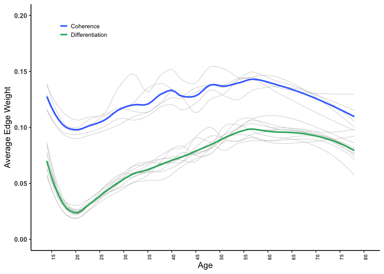

(#fig:diff coh plots)Figure 1. Coherence (green) and differentiation (blue) across the lifespan. Coherence is indicated by higher average inter-item partial correlations within scales, while differentiation is indicated by lower average-inter-item partial correlations across sub-scales of the Big Five. Thus, increases in the blue differentiation line indicate decreases in differentiation and vice versa. Light gray lines show the unique trajectory for each of the Big Five.

# ggsave(sprintf("%s/photos/differentiation_coherence_line_graph.png", data_path), 
#        width = 5, height = 4)

6.2 Single and Mutli-Trait Coherence

edges.sum %>%
  full_join(trait.edges.sum) %>%
  filter(comp != "Differentiation" & inventory == "IPIP50") %>%
  ggplot(aes(x = as.numeric(age), y = mean, group = comp)) + 
      geom_line(data = filter(edges.sum, comp == "Coherence" & inventory == "IPIP50"), aes(color = Trait, linetype = type)) + 
      geom_line(data = trait.edges.sum %>% filter(inventory == "IPIP50"), aes(color = Trait, linetype = type)) + 
      scale_x_continuous(limits = c(14,80), breaks = seq(15, 80,5)) + 
      scale_linetype_manual(values = c("dotted", "solid")) +
      guides(color = F) +
      facet_wrap(~Trait, nrow = 3) + 
      labs(x = "Age", y = "Average Edge Weight", color = "Big5\nTrait", linetype = "Network\nType") + 
      theme_classic() + 
      theme(axis.text.x = element_text(size = rel(.5), face = "bold", angle = 90),
            axis.text.y = element_text(face = "bold"),
            legend.position = c(.75,.15),
            legend.key.size = unit(.5, "cm"), 
            legend.text = element_text(size = rel(.75)),
            legend.title = element_text(size = rel(.75), face = "bold"))

## Joining, by = c("inventory", "age", "traits", "comp", "mean", "type", "gmean", "Trait")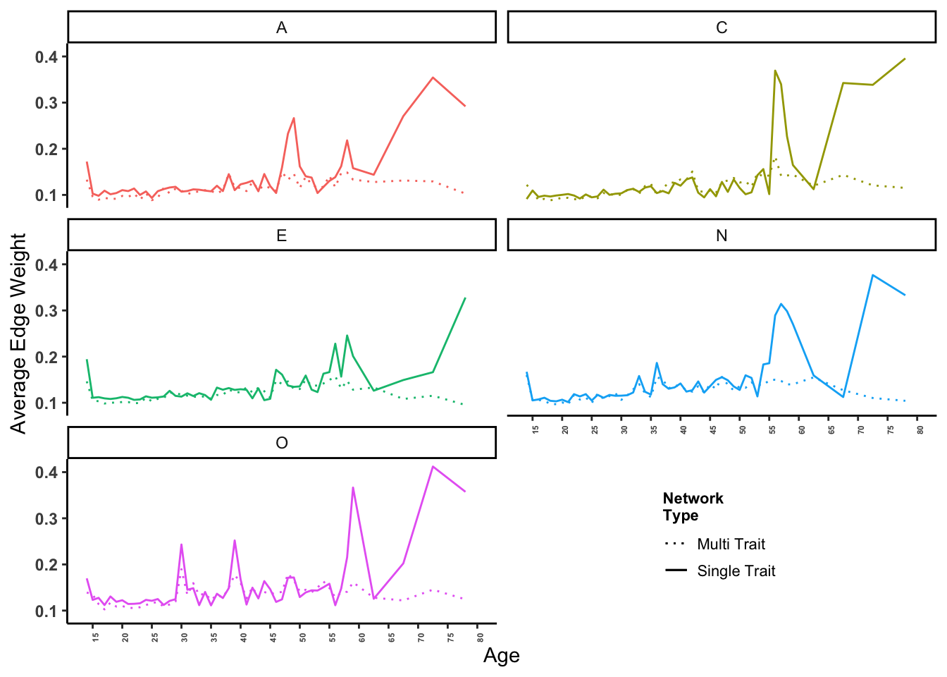

(#fig:st coherence plot)Figure 2. Coherence across the lifespan by trait. Solid lines indicate coherence when each trait was modeled separately, while dotted lines indicate coherence when the full IPIP-50 Big Five scale was modeled simultaneously. Coherence is indicated by higher average inter-item partial correlations within scales; thus increases in coherence across age groups suggests increasing coherence.

# ggsave(sprintf("%s/photos/by_trait_differentiation_coherence_line_graph.png", data_path), 
#        width = 5, height = 4)