Chapter 8 Profile Correlations
Next, we calculate profile correlations to test the stability of edges across all possible pairwise combinations of ages. A strong parallel correlation indicates that the weight of the edges is associated across two ages. We then map these profile correlations onto a heat map that displays the pairwise profile correlations. We would expect to see the strongest profile correlations cluster on the diagonal of heatmap – that is between ages that are adjacent or near in age.
## Multi-Trait
wide_fun <- function(df){
  df <- unclass(df) %>% data.frame %>%
    select(-from, -to) %>% spread(key = edge, value = weight)
  rownames(df) <- df$age
  df <- df %>% select(-age)
  return(df)
  }

# change the direction of the data
MT_procor <- MT_net_nested %>%
  unnest(edges.df) %>%
  group_by(inventory) %>%
  nest() %>%
  mutate(wide = map(data, wide_fun),
         procor = map(wide, ~cor(t(.), use = "pairwise.complete.obs")))

# separate out differentiation from coherence
edges.mat50bw <- MT_net_nested %>%
       filter(inventory == "IPIP50") %>% unnest(edges.df) %>%
       separate(from, into = c("from_factor", "from_item"), 1) %>%
       separate(to, into = c("to_factor", "to_item"), 1) %>%
       filter(from_factor != to_factor) %>%
       select(age, weight, edge) %>%
       spread(key = edge, value = weight) %>%
       unclass %>% data.frame

# separate out coherence from differentiation
edges.mat50wi <- MT_net_nested %>%
       filter(inventory == "IPIP50") %>% unnest(edges.df) %>%
       separate(from, into = c("from_factor", "from_item"), 1) %>%
       separate(to, into = c("to_factor", "to_item"), 1) %>%
       filter(from_factor == to_factor) %>%
       select(age, weight, edge) %>%
       spread(key = edge, value = weight) %>%
       unclass %>% data.frame

# set the rownsames of these to age
rownames(edges.mat50bw) <- edges.mat50bw$age
rownames(edges.mat50wi) <- edges.mat50wi$age

##############################################
############ Profile Correlations ############
##############################################

# calculate profile correlations
procor50bw <- cor(t(edges.mat50bw[,-1]), use = "pairwise.complete.obs")
procor50wi <- cor(t(edges.mat50wi[,-1]), use = "pairwise.complete.obs")
8.1 Profiles Correlation Plots (Figure 5)
##############################################
################## PLOTS #####################
##############################################

procor_plot_fun <- function(df, inv, leg){
  df[upper.tri(df, diag = T)] <- NA
  p <- tbl_df(df) %>%
    mutate(age1 = colnames(.)) %>%
    gather(key = age2, value = r, 1:(ncol(.) - 1)) %>%
    filter(!is.na(r)) %>%
    ggplot(aes(x = age2, y = age1, fill = r)) +
      geom_raster(aes(fill = r)) +
      scale_fill_gradient2(low = "blue", high = "red", mid = "white",
       midpoint = .5, limit = c(0,1), space = "Lab",
       name="Profile\nCorrelation") +
      labs(x = "Age", y = "Age", title = sprintf("Profile Correlations for %s", inv)) +
      theme_classic() +
      theme(legend.position = leg,
            axis.text = element_text(face = "bold"),
            axis.text.x = element_text(angle = 90, size = rel(.8)),
            plot.title = element_text(hjust = .5))
  # ggsave(p, file = sprintf("%s/photos/Big5_%s_profile_cors_heatmap.png", data_path, inv), width = 12, height = 8)
  p
}

MT_procor <- MT_procor %>%
  mutate(plot = map2(procor, inventory, ~procor_plot_fun(.x, .y, leg = "none")))

layout <- rbind(c(1, 1, 2),
                c(1, 1, 3))
p <- gridExtra::grid.arrange(
  MT_procor$plot[[2]],
  procor_plot_fun(procor50bw, "IPIP50 Cross-Trait Edges", leg = "none"),
  procor_plot_fun(procor50wi, "IPIP50 Within-Trait Edges", leg = "none"),
  layout_matrix = layout)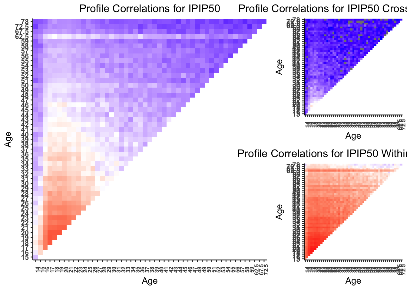
# ggsave(p, file = sprintf("%s/photos/Big5_IPIP50_profile_cors_heatmap.png", data_path),
       # width = 12, height = 8)
rm(list = ls())